Visualization with OpenDX

The objective of this assignment is to visualize a 2D dataset using OpenDX.

OpenDX is an extremely powerful data visualization tool. The downside is the steep learning curve. In this homework, you will create a vision of a 2D dataset with a few extra options.

Task 1: Create the dataset.

Second part: Let's assume that the DLA aggregate is an electrode in a petri dish and compute the electrostatic potential for this arrangement. Still in cimage, choose Special and Potential Operator. In the dialog, leave everything untouched except SOR, which you set to 1.8. Hit OK to start. Since by default the inner electrode is ground, invert the resulting image. The center (of the approximate shape of the DLA) should now be white. Save this image both as TIFF and as DX.

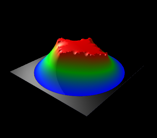
Visualize this image as 3D surface using cimage. Use Special, then 3D surface view (GL). Increase Z scale and turn on spotlight illumination. Your rendering should look like the image below. Save the scene image with a ".png" suffix, for example dla_scene.png.

Alternatives: You may choose alternative "scenes" to visualize as long as it encompasses the merging of two distinct parts (as in the example above the DLA cluster and its potential field). A color bar should be included. Some suggested examples:

• A grayscale mountainscape (e.g., Perlin noise) with the image value rendered as height. At some level, the mountainscape is submerged and under water. The water may be semitransparent and parts of the submerged mountainscape could still be visible. Use a suitable "natural" color map and include contour lines.
• A sequence of 2-3 visions of the sum of two Gaussian functions, their center highlighted by a cylinder or disc; as the centers get closer than their FWHM, the vision should make obvious why the individual centers can no longer be separated. Highlight the level of the FWHM.

Task 2: Create the vision with OpenDX.

For the example above, the result should look as follows:

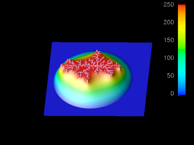
Note how the DLA cluster (in white) is superimposed over the electrostatic potential level, and how a colorbar has been added. If you choose your own scene, similar features should exist.

Hints and tricks:

• A module called Colorbar exists in OpenDX. Use it together with Collect to add the colorbar to the image.
• Rather than using Autocolor, combine Colormap and Color to false-color the dataset. Use the output of Colormap as input for Colorbar.
• For Task 3, you will need a third input to Collect. Click on the module, then go to Edit -> Input/output tabs and choose Add input tab.
• Once again, use Colormap and Color to add color to the DLA cluster. This time, however, you need to make the background transparent. Wire both outputs of Colormap to the first and second input of Color, respectively, to provide an opaqueness (alpha) channel. Create a suitable colormap that adds white color to the maximum values and minimum opacity to the minimum values. At this time, the DLA is at the bottom of the potential mountain.
• You still have to map the DLA cluster to the 3D surface of the potential surface. This is a bit tricky, so here is a recipe: Add a Compute module and wire the output of the DLA Color module to the first Compute input. Add a Mark module and wire the output of the Rubbersheet from the potential mountain through Mark into the second input of Compute. Wire the output of Compute into an Unmark module and from there into the third Collect input. Double-click on Mark and choose "positions" for the name input. Do the same with Unmark. Finally, double-click Compute and add the formula to compute: [b.x, b.y, b.z+1]. This way, you use the positions from the rubbersheet to elevate the DLA cluster. Except that you let the DLA hover a little bit above the mountain (with b.z+1) to render it more clearly.

Due date

The homework is due on 05/05/16 in by e-mail.