Continued from part 1.
|
|
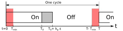
| Figure 1: Diagram of an on-off cycle of duration $T$. At the start of each cycle, the furnace or compressor is turned on and stays on for a duration of $T_0 + k_p \cdot \epsilon$. The red zones are cutoff zones where a cycle is either skipped or continued into the next to reduce startup stress. |
How do we choose $k_p$? First, it is advantageous to re-interpret the on-time $T_{on}$ as a fraction of $T$: $$ T_{on} = T \cdot \left( P_0 + k_p \cdot \epsilon \right) $$ Here, $P_0 = T_0 / T$ is the base on-time as a fraction of the cycle time $T$, and $k_p$ is also seen as a fraction of $T$, meaning, $k_p$ has units of inverse degrees C under this definition. A good value of $k_p$ needs to be determined experimentally. I started with adding approximately 15% of the cycle duration $T$ per degree of control deviation. This value turned out to be too low, whereby the temperature takes a long time to equilibrate. Choosing a very high value of $k_p$ leads to undesirable behavior as the thermostat fluctuates between staying on too long and skipping a cycle. In the end, I settled on values between $k_p=0.2$ and $k_p=0.25$.
It is interesting to observe that the air conditioning requires much larger values of $k_p$. To get acceptable cooling behavior, I settled on $k_p=0.4$. The cause is the lower "gain" of the cooling unit: the furnace can raise the temperature almost twice as fast as the compressor can reduce the temperature by the same amount.
One special consideration is necessary. If the on-time $T_{on}$ is very close to zero or very close to $T$, it does not make sense to turn on the furnace or A/C unit for a few seconds (or turn them off for a few seconds between cycles). For the compressor, start-up stress is a major consideration. The furnace, on the other hand, follows a lengthy sequence of functions: first, it purges the air for 90 seconds to remove any potential leaked gas. Only then the flame is ignited. Both heating and cooling functions keep the main blower running for about a minute to clear the air ducts. It is reasonable to create a cutoff: If $T_{on} < T_{min}$, a cycle is skipped entirely. Conversely, if $T_{on} > T - T_{min}$, the HVAC is kept on through the next cycle, but a measurement is taken at the start of the cycle. These cutoff limits are shown in red in Figure 1. In practice, I chose $T_{min}=180$s as this is the shortest time that allows some noticeable heating action.
In the discrete world, the integral turns into a sum, that is, $$ \int_{t_0}^{t_1} f(t) \textrm{d}t \approx \sum_k f_k \cdot \Delta t $$ where $f(t)$ is a continuous function and $f_k = f(k \Delta t) \cdot \delta (t - k \Delta t)$ is the discrete sequence of function values sampled on integer multiples of the sampling interval $\Delta t$. To obtain an integral component, we can therefore sample the residual control deviation at the end of each cycle and accumulate it. Thus, we obtain the integral correction $T_I$ as $$ T_I = k_I \cdot T \cdot \sum_k \epsilon_k $$ where $k_I$ is the integral gain, which is usually chosen to be a very small value.
We can interpret $T_I$ as another time component that gets "tacked on" to the on-time and that depends on a repeated, systematic deviation of the temperature. For example, if the room is consistently too cold after heating stops, $T_I$ slowly increases. If we use for $T_{on}$ $$ T_{on} = T \cdot \left( P_0 + k_p \cdot \epsilon + k_I \sum_k \epsilon \right) $$ we can see that the on-time would slowly increase over time, thus correcting for the shortfall. In practice, it is straightforward to adjust $P_0$ at the end of each cycle by $k_I \epsilon$. In this fashion, $P_0$ dynamically adjusts and therefore carries the integral component.
|
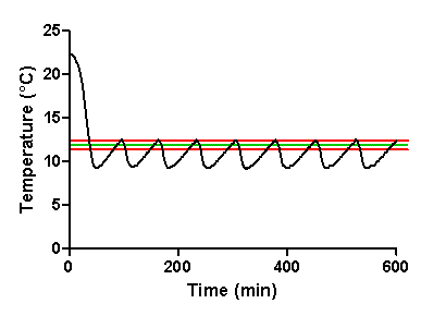
| Figure 2: Cooling behavior of a fridge/freezer with conventional two-point control. the green line is the setpoint, and the red lines represent the lower and upper trip points of the two-point control. The fridge starts equilibrated to room temperature. Strong temperature swings appear as cold air from the freezer compartment diffuses into the fridge compartment. |
|
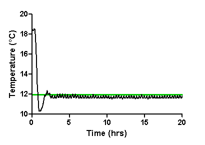
| Figure 3: Cooling behavior of a fridge/freezer with the proposed pseudo-linear control system. The green line indicates the setpoint. The fridge starts equilibrated to room temperature. Unlike two-point control, the new system creates a very accurate estimate of the run-time to keep temperature fluctuations at a minimum. However, the compressor switches more frequently than in the two-point system in Figure 2. |
With the new system, as described above, temperature fluctuations are dramatically decreased (Figure 3), although overshoot is still present when a large temperature difference needs to be traversed. However, the superior control accuracy becomes evident.
With the proof of principle established, how can we design such a thermostat for one's home? This is not as bad as it sounds, because most of the functions can be done in software and the overall electronic circuit remains relatively simple. So... on to Part 3.